Image processing with pillow and NumPy
To be frank, I had heard from various sources that “images are just arrays,” and I used to nod along until I actually got into working with NumPy. And guess what? I had no clue whatsoever.When I looked at an image, I saw a picture. My brain processed it as a whole thing a cat, a face, a sunset. But NumPy doesn't see any of that. NumPy sees a table of numbers. And the moment I truly accepted that, everything clicked.
Wanna learn the basics?
Check out my repository here: https://github.com/Mominulcse11/Numpy
Images Are Matrices
In computer science, an image is just a grid of numbers representing pixels.
Grayscale (2D Array): Shape: (Height, Width)Data:Represented by a single 2D grid. Each number represents the light intensity (or brightness) of that pixel, typically ranging from [0(pure black) , 255 (pure white)]
RGB (3D Array): Shape: (Height, Width, 3) Data:Represented by three overlapping 2D grids (channels) stacked on top of each other, usually for Red, Green, and Blue (RGB). Each pixel is a combination of these three values, allowing for millions of possible colors
RGBA (3D Array): Shape: (Height, Width, 4) Data: Includes the three RGB channels plus a 4th Alpha channel for transparency (0 is fully transparent, 255 is fully opaque).
RGB Structure
Every pixel in a color image is a triplet — [R, G, B]. Three numbers, each between 0 and 255.
So img_array[0, 0] gives you the top-left pixel. Something like [255, 230, 180]. That's almost white with a warm tint.
The axes mean:
axis 0 → rows (height, top to bottom)
axis 1 → columns (width, left to right)
axis 2 → channels (R, G, B)
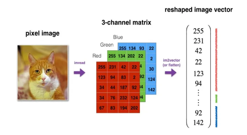
PIL (Pillow) library and NumPy to load and inspect an image:
import numpy as np
import matplotlib.pyplot as plt
from PIL import Image

img = Image.open("cat.jpg")
print(type(img))
img_array = np.array(img)

print(img_array.shape)
Output: (148, 269, 3)
148 rows. 269 columns. 3 color channels. That's your Meow.
A quicck check whats going on to the display:
plt.imshow(img_array)
plt.show()
Output:
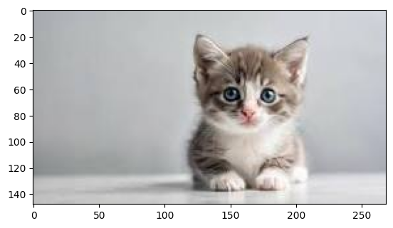
The function plt.imshow() converts the matrix into a color map.It prepares the imageplt.show() displays the image on the display.
crop
Cropping an image is just array slicing:
crop = img_array[100:140, 50:250]

plt.imshow(crop)
plt.show()
print(img_array.shape)
Output:
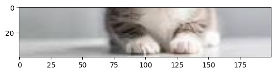
like you are saying give me rows 100 to 140, columns 50 to 250.General pattern is img_array[row_start:row_end, col_start:col_end]
Flipping
Horizontal flip — reverse the columns:
horflipped = img_array[:, ::-1]

plt.imshow(horflipped)
plt.show()
Output:
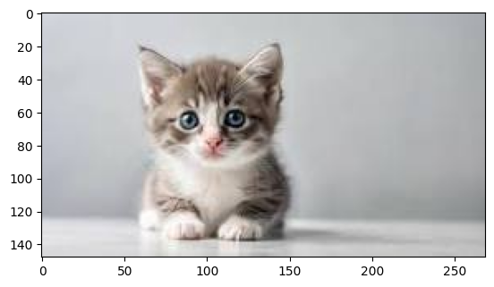
: (First dimension): Selects all rows.
::-1: Selects all columns but steps backward by 1. This reverses the horizontal order of pixels.Slice notation generally follows the format [start:stop:step]
Vertical flip — reverse the rows:
verflipped = img_array[::-1, :]

plt.imshow(verflipped)
plt.show()
Output:
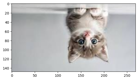
Same idea.But on axis 0.The image flips Upside DOwn like Hawkins.
Rotation
Rotation is bit more interesting .Cuz there is no single step slice for this
you need to use transpose first .Then flipping columns give rotation.
transpose = img_array.transpose(1, 0, 2)

rotate = transpose[:, ::-1]
plt.imshow(rotate)
plt.show()
Output:
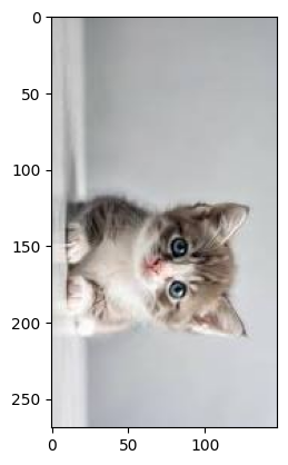
Why (1, 0, 2)?
axis 1 becomes the new first axis
axis 0 becomes the new second axis
axis 2 (RGB) stays where it is
So (H, W, 3) becomes (W, H, 3) .Then nedd flip the columns.
Tiny Experiments
The real learning happens when you break things on purpose.
Brighten the image:
bright = img_array + 50
bright = np.clip(bright, 0, 255)

plt.imshow(bright)
plt.show()
Output:
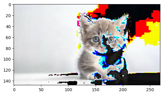
Use clip cuz pixel range [0,250]
Isolate the red channel:
redd = img_array.copy()
redd[:, :, 0] = 0  # zero out red
redd[:, :, 1] = 0  # zero out green

plt.imshow(redd)
plt.show()
Output:
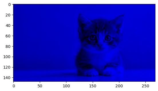
Using masking here — selectively zeroing out channels. Only red survives.
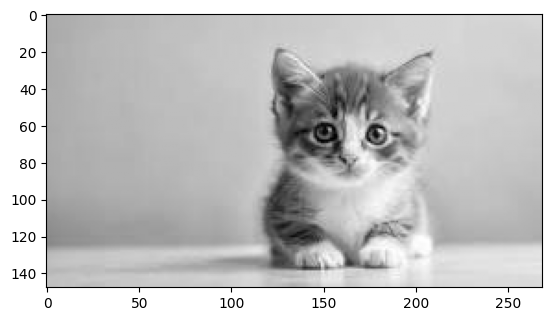
Convert to grayscale:
RGB image:3 channels
Grayscale:1 intensity value
Luminosity (Weighted) Method: This is the most accurate method because it accounts for human visual perception—our eyes are most sensitive to green, then red, and least to blue. Formula: 0.299R+0.587G+0.114B
Average Method: Simply averages the three channels. It is easier to calculate but may result in less visual depth.Formula: (Gray = R + G + B\3)
Data Compression: Grayscale images use only 8 bits per pixel (one channel) compared to 24 bits for RGB (three channels), significantly reducing file size. Image Processing: Many complex algorithms (like edge detection or face recognition) work faster and more reliably on single-channel grayscale data.
gray = np.dot(
    img_array[..., :3],
    [0.299, 0.587, 0.114]
)

plt.imshow(gray, cmap='gray')
plt.show()
output:
blur
Its the most interesting experiment.
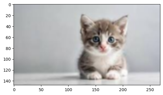
Blur is conceptually simple also not simple: replace each pixel with the average of its nearby pixels.
he more neighbors you include, the more blurred it gets. That neighborhood is called a kernel. A 3×3 kernel looks at 9 pixels around each point. A 5×5 looks at 25.
blurred = img_array.copy()

for i in range(1, img_array.shape[0]-1):
    for j in range(1, img_array.shape[1]-1):

        blurred[i, j] = np.mean(
            img_array[i-1:i+2, j-1:j+2],
            axis=(0,1)
        )

plt.imshow(blurred.astype(np.uint8))
plt.show()
output:
Blur is conceptually simple: replace each pixel with the average of its nearby pixels.
he more neighbors you include, the more blurred it gets. That neighborhood is called a kernel. A 3×3 kernel looks at 9 pixels around each point. A 5×5 looks at 25.
Try these yourself:
- Flip the image vertically
- Isolate only the green channel
- Rotate the image counterclockwise
- Brighten only the top half of the image
- Make a black and white mask where red > 150